7 Linkage to Exposures


Linking Geocoded Addresses to Various Geospatial Exposure Types Using NIEHS Tools in R
Date Modified: August 10, 2023
Authors: Lara P. Clark ![]() , Kyle P. Messier
, Kyle P. Messier ![]() , Sue Nolte, Charles Schmitt
, Sue Nolte, Charles Schmitt ![]() et al.
et al.
Key Terms: Data Integration, Exposure, Exposure Assessment, Geocoded Address, Geospatial Data
Programming Language: R
7.1 Introduction
7.1.1 Motivation
Climate change and health research draws upon diverse types of open geospatial data to assess individuals’ environmental exposures, such as exposure to air pollution, green space, and extreme temperature. Calculating such environmental exposures using open geospatial data can be challenging and can require expertise from multiple disciplines, from geographic information science to exposure science to bioinformatics. Open source software can help reduce barriers and support broader use of open geospatial data for assessing environmental exposures using reproducible methods.
7.1.2 Approach
This chapter describes NIEHS open source tools to link environmental exposures to individual health data based on geocoded addresses (i.e., geographic coordinates, latitude and longitude). These tools are intended to be accessible to researchers without training in geographic information science (GISc) or geographic information systems (GIS) software. These tools require basic or beginner level programming in R.
The tools consist of code, standardized data, and documentation describing use for environmental health applications. Each tool calculates a selection of environmental exposure metrics based on a different source of open geospatial data with national (or approximately national) coverage for United States. Exposure metrics are calculated based on specified point locations (i.e., geocoded address or other geographic coordinates). For data sources that include temporal information, the exposure metrics are also calculated based on specified times. Output of the tool includes the calculated exposure metrics as well as information about data missingness and an optional log file. These tools are designed to be run completely offline as an approach to protect personal geolocation data (Brokamp 2018).
These tools depend on the following R packages: sf (Pebesma 2018; Pebesma and Bivand 2023), terra (Hijmans 2024), and tidyverse (Wickham et al. 2019).
7.1.3 Tools
The following summarizes the available tools and planned tools:
| Tool | Exposure Metrics | Spatial Details | Temporal Details | Status |
|---|---|---|---|---|
| Air pollution (CACES model) | Annual average outdoor concentrations of ozone, particulate matter (PM2.5, PM10), sulfur dioxide, carbon monoxide, and nitrogen dioxide air pollution | Census tracts in the contiguous US | Yearly during 1979-2015 (varies by pollutant) | Version 1.0 |
| Airport proximity | Distance to nearest, number within buffer distance, summary of distances (mean, mean of log, 25th, 50th and 75th percentiles) within buffer distance | Points in the US | Yearly during 1981-2020 | Version 1.0 |
| Major road proximity | Distance to nearest, length in buffer distance | Lines in the US | Yearly during 2000-2018 | Version 1.0 |
| Air pollution (ACAG model) | Annual average outdoor concentrations of particulate matter (PM2.5) and its components | 0.01 degree grid in North America | Yearly during 2000-2018 | In Development |
| Superfund sites | Distance to nearest, number within buffer distance, summary of distances (mean, mean of log, 25th, 50th and 75th percentiles) within buffer distance | Points in the US | 2014 | In Development |
7.1.4 Additional Resources
Other available tools to calculate environmental exposures for health applications:
- DeGAUSS geomarker software (Brokamp 2018) provides containerized tools to calculate various geospatial exposure metrics based on geocoded address and state and end date. These metrics include proximity to roadways, traffic, land cover, and vegetation indices.
7.2 CACES Air Pollution
The following are step-by-step instructions to calculate annual average air pollution exposure metrics using the Center for Air, Climate, & Energy Solutions (CACES) land use regression models (Version 1.0).
7.2.1 Description
CACES Air Pollution Model Data
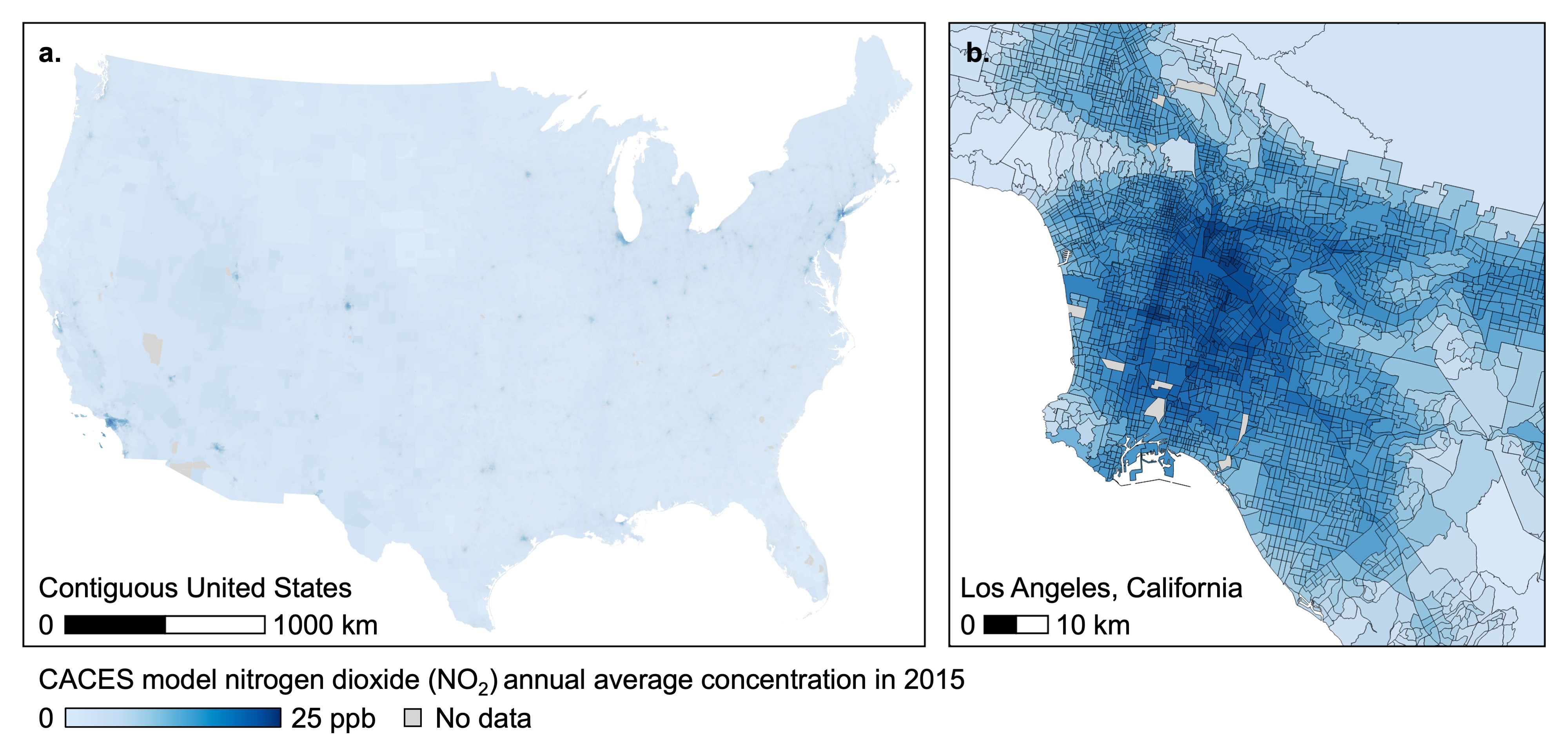
The CACES models are based on air pollution observations from United States (US) Environmental Protection Agency monitors and from satellites, as well as land cover and land use information (e.g., locations of roadways). CACES model predictions cover populated locations in the contiguous US (i.e., in the 48 contiguous states plus the District of Columbia) at the spatial resolution of US census tracts, for the following air pollutants and time-periods:
| Air pollutant | Units | Exposure metric | Available years |
|---|---|---|---|
| carbon monoxide (CO) | ppm | annual average concentration | 1990-2015 |
| nitrogen dioxide (NO2) | ppb | annual average concentration | 1979-2015 |
| ozone (O3) | ppb | May through September average of daily moving 8-hour maximum average concentration | 1979-2015 |
| particulate matter (PM2.5) | µg m-3 | annual average concentration | 1999-2015 |
| particulate matter (PM10) | µg m-3 | annual average concentration | 1988-2015 |
| sulfur dioxide (SO2) | ppb | annual average concentration | 1979-2015 |
The following figure illustrates the spatial coverage (contiguous US) and spatial resolution (census tracts) for a single pollutant and time-period (NO2 in 2015):
Exposure Metrics
This tool calculates long-term average air pollution exposure metrics for a specified list of receptor point locations (e.g., geocoded home addresses) during a specified time-period in years. This tool can be used to calculate average exposure metrics:
- for a single year or single range of years that is constant across all receptor locations (e.g., 2002, 2010 to 2015)
- for a single year or range of years that varies across receptor locations (e.g., year of birth, years of residence at geocoded home address)
Exposure metrics can be calculated for all CACES pollutants or any subset of them. Output includes information about data missingness (e.g., whether a specified receptor point is located outside the coverage of the CACES data) as well as an optional log file.
Recommended Uses
This tool is recommended for the following uses:
- Comparisons of exposures across larger geographic regions in the contiguous US (e.g., across a metropolitan area or state). Note: This tool is based on census tract level air pollution model data and cannot be used to compare exposures for different locations within the same census tract.
- Comparisons of exposures incorporating multiple pollutants and/or years in
a consistent manner
- Analyses focused on long-term average (e.g., annual average, multi-year average) exposures to air pollution
7.2.2 Install R and Required Packages
Install R. Optionally, install RStudio.
Then, install the following R packages: logr, tidyverse, sf.
Follow R package installation instructions, or run the following code in R:
7.2.3 Download Tool
Download and save the folder containing input data (input_source_caces.rds and input_census_tracts_2010.rds) and script (script_caces_exposures_for_points.R). To directly run the example scripts provided with these instructions in Step 4, do not change the file names within the folder.
7.2.4 Prepare Receptor Point Data
Prepare a comma-separated values (CSV) file that contains a table of the receptor point locations (e.g., geocoded addresses, coordinates). Include each receptor as a separate row in the table, and include the following required columns:
id: a unique and anonymous identifying code for each receptor. This can be in character (string) or numeric (double) format.idmust be unique across all rows in the receptor point location table. It is not possible to use the sameidfor different time-points or locations within the same receptor point location table.
latitude: the latitude of the receptor point location in decimal degrees format (range: -90 to 90)longitude: the longitude of the receptor point location in decimal degrees format (range: -180 to 180)
To calculate exposure metrics for time-periods (year or range of years) that vary across the receptors (e.g., years of residence at geocoded addresses), include both of the following optional columns:
time_start: the first year of the time-period in “YYYY” format (e.g.,2002for year 2002)
time_end: the last year of the time-period in “YYYY” format (e.g.,2003for year 2003)
To calculate exposure metrics for a single year that varies across the receptors, provide the same year for both time_start and time_end for each receptor. To calculate exposure metrics for a range of years that is constant across the receptors, provide the start year of the range as time_start for all receptors and the end year of the range as time_end for all receptors. To calculate exposure metrics for a single year that is constant across all receptors, specify year for exposure assessment using argument caces_year. If both caces_year and time_start and time_end are provided, the exposure assessment will be based on caces_year (ignoring time_start and time_end).
The following table provides an example of the receptor point data format:
| id | latitude | longitude | time_start | time_end |
|---|---|---|---|---|
| 1011A | 39.00205369 | -77.105578716 | 2002 | 2011 |
| 1012C | 35.88480215 | -78.877942573 | 2014 | 2015 |
| 1013E | 39.43560788 | -77.434847823 | 1990 | 1990 |
To directly run the example scripts provided with these instructions, save the receptor point data as input_receptor.csv in the folder.
7.2.5 Run Script in R
Run the script script_caces_exposures_for_points.R to load the required functions
in R. You can then use the function get_caces_for_points() to calculate
the mean CACES model pollutant concentrations for the selected time period (in years)
for each receptor point location.
Description of Function get_caces_for_points()
This function takes the receptor point data above and returns a data frame with the receptor id linked to the exposure estimates for selected pollutants and time periods as well as information about data missingness. Optionally, the function also writes a log file in the current R working directory. The function has the following arguments:
Required Arguments
receptor_filepath: specifies the file path to a CSV file containing the receptor point locations (described in Step 3). Note: The format for file paths in R can vary by operating system.
source_caces_filepath: specifies the file path to a RDS file containing a data frame with the CACES air pollution estimates by census tract. This is the fileinput_source_caces.rds.
source_census_tracts_2010_filepath: specifies the file path to a RDS file containing the simple features with the 2010 census tracts for the US. This is the fileinput_census_tracts_2010.rds.
Optional Arguments
receptor_crs: a coordinate reference system object (i.e., class iscrsobject in R) for the receptor point locations. Default is “EPSG:4269” (i.e., NAD83).caces_pollutants: list that specifies the subset of CACES pollutants to include. Default is all pollutants:"co", "no2", "o3", "pm10", "pm25", "so2".
caces_year: specifies a single year (in “YYYY” format; e.g., 2003) for exposure assessment across all pollutants and receptors. Default isNULL.caces_yearis required to be specified iftime_startandtime_endare not provided with the receptor point data. If bothcaces_yearandtime_startandtime_endare provided, exposure assessment will be based on the single year specified bycaces_year(i.e., ignoringtime_startandtime_end).caces_yearmust beNULLif usingtime_startandtime_endto specify year(s) that vary across receptor points for exposure assessment.caces_yearmust be during 1999-2015 to return exposure estimates for all six pollutants, or during 1979-2015 for O3, NO2, and SO2, 1988-2015 for PM10, 1990-2015 for CO, or 1999-2015 for PM2.5.
add_all_input_to_output: logical argument that specifies whether the output should include all columns included with receptor point locations (described in Step 3).TRUEreturns all columns (i.e., including any time information and census tract identifying code) with output.FALSEreturns only the anonymous receptor identifying code, exposure estimates, and data missingness flags with output.FALSEmay be useful for meeting data de-identification requirements. Default isTRUE.
write_log_to_file: logical argument that specifies whether a log should be written to file.TRUEwill create a log file in the current working directory. Default isTRUE.
print_log_to_console: logical argument that specifies whether a log should be printed to the console.TRUEwill print a log to console. Default isTRUE.
Example Use
Below are two example scripts for using the function above to produce a CSV file with the CACES exposure estimates for each receptor point for ozone and nitrogen dioxide in year 2015 (using default options for all other optional arguments). The first example uses only R but requires editing the file paths. The second example requires RStudio and the here package but does not require editing file paths.
Example 1: Base R
# Load packages
library(tidyverse)
library(logr)
library(sf)

# Load functions
source("/set/file/path/to/script_caces_exposures_for_points.R")

# Get exposures
caces_exposures <-
  get_caces_for_points(
    receptor_filepath = "/set/file/path/to/input_receptor.csv",
    source_caces_filepath = "/set/file/path/to/input_source_caces.rds",
    source_census_tracts_2010_filepath =
    "/set/file/path/to/input_census_tracts_2010.rds",
    caces_year = 2015,
    caces_pollutants = c("o3", "no2")
  )

# Write exposures to CSV
readr::write_csv(caces_exposures,
  file = "/set/file/path/to/output_caces_exposures.csv"
)
Example 2: RStudio with here Package
# Install here package (if needed)
install.packages("here")

# Load packages
library(here)
library(tidyverse)
library(logr)
library(sf)

# Set location
here::i_am("script_caces_exposures_for_points.R")

# Load functions
source(here::here("script_caces_exposures_for_points.R"))

# Get exposures
caces_exposures <-
  get_caces_for_points(
    receptor_filepath = here("input_receptor.csv"),
    source_caces_filepath = here("input_source_caces.rds"),
    source_census_tracts_2010_filepath =
    here("input_census_tracts_2010.rds"),
    caces_year = 2015,
    caces_pollutants = c("o3", "no2")
  )

# Write exposures to CSV
readr::write_csv(caces_exposures,
  file = here("output_caces_exposures.csv")
)
7.2.6 Review Output
Log File
After running the example script above, with the log file option selected, the log
file will be available in the folder log in the current R working directory.
Output Data
After running the example script above, calculated exposure metrics for receptor
locations will be available in the file output_caces_exposure.csv within the
folder. This CSV file includes a row for each receptor with the following columns (as applicable):
Identifiers
id: the unique and anonymous identifying code for each receptor
fips_tr_10: the identifying code (FIPS code) for the year 2010 census tract
Calculated Exposure Metrics
co: mean CACES model predicted concentration of outdoor annual average carbon monoxide (CO) air pollution (units: parts per million [ppm]) for the census tract that contains the receptor point location during the specified year(s)
no2: mean CACES model predicted concentration of outdoor annual average nitrogen dioxide (NO2) air pollution (units: parts per billion [ppb]) for the census tract that contains the receptor point location during the specified year(s)
o3: mean CACES model predicted concentration of outdoor annual average ozone (O3) air pollution (units: parts per billion [ppb]) for the census tract that contains the receptor point location during the specified year(s)
pm25: mean CACES model predicted concentration of outdoor annual average particulate matter (PM2.5) air pollution (units: micrograms per cubic meter [µg m-3]) for the census tract that contains the receptor point location during the specified year(s)
pm10: mean CACES model predicted concentration of outdoor annual average particulate matter (PM10) air pollution (units: micrograms per cubic meter [µg m-3]) for the census tract that contains the receptor point location during the specified year(s)
so2: mean CACES model predicted concentration of outdoor annual average sulfur dioxide (SO2) air pollution (units: parts per billion [ppb]) for the census tract that contains the receptor point location during the specified year(s)
Information on Data Missingness
caces_flag_01: binary variable indicating whether the receptor point is located within a year 2010 US census tract:1indicates that receptor point is not located within a year 2010 US census tract. All exposure metrics for that receptor point will be reported asNA.0indicates that receptor point is located within a year 2010 US census tract
caces_flag_02: binary variable indicating whether receptor point is located within a year 2010 US census tract but outside the spatial coverage of the CACES air pollution model:1indicates receptor point is located within a year 2010 US census tract but outside the spatial coverage of the CACES air pollution model. Examples include tracts in Alaska, Hawaii, or US territories, and tracts with no population recorded in the 2010 Decennial Census. All exposure metrics for that receptor point will be reported asNA.
0indicates that receptor point is located within a year 2010 census tract within coverage of the CACES air pollution model
caces_flag_03: binary variable indicating whether the specified time period for that receptor point is completely outside the coverage of the CACES air pollution model:1indicates that the specified time (year(s)) for that receptor point is completely outside the temporal coverage of CACES air pollution model for one or more of the selected pollutants. Exposure metrics will be reported asNAfor one or more of the selected pollutants.
0indicates that the specified time (year(s)) for that receptor point is not completely outside the temporal coverage of CACES air pollution model for any of the selected pollutants
caces_flag_04: binary variable indicating whether the specified time-period (year(s)) for that receptor point is partly outside the temporal coverage of CACES air pollution model for one or more of the selected pollutants.1indicates that the the specified time-period (year(s)) for that receptor point is partly outside the temporal coverage of CACES air pollution model for one or more of the selected pollutants. Exposure metrics will be calculated based on the years with available data for that specified time-period.
0indicates that the specified time-period (year(s)) for that receptor point is completely within the temporal coverage of CACES air pollution model for all of the selected pollutants.
7.2.7 Cite Data and Tool
Please cite the following in any publications based on this tool:
CACES Empirical Air Pollution Models (v1):
Kim S.-Y.; Bechle, M.; Hankey, S.; Sheppard, L.; Szpiro, A. A.; Marshall, J. D. 2020. “Concentrations of criteria pollutants in the contiguous U.S., 1979 – 2015: Role of prediction model parsimony in integrated empirical geographic regression.” PLoS ONE 15(2), e0228535. DOI: 10.1371/journal.pone.0228535
Census Tract Spatial Boundaries:
Steven Manson, Jonathan Schroeder, David Van Riper, Tracy Kugler, and Steven Ruggles. IPUMS National Historical Geographic Information System: Version 16.0 [Census Tract Shapefiles, 2010]. Minneapolis, MN: IPUMS. 2021. http://doi.org/10.18128/D050.V16.0
Please see the following for additional requirements: https://www.nhgis.org/citation-and-use-nhgis-data
NIEHS Geospatial Toolbox:
Citation to be determined.
7.3 Airport Proximity
The following are step-by-step instructions to calculate proximity-based exposure metrics to aircraft landing facilities in the United States (US) using Federal Aviation Administration (FAA) aircraft landing facility data.
7.3.1 Description
FAA Aircraft Landing Facility Data
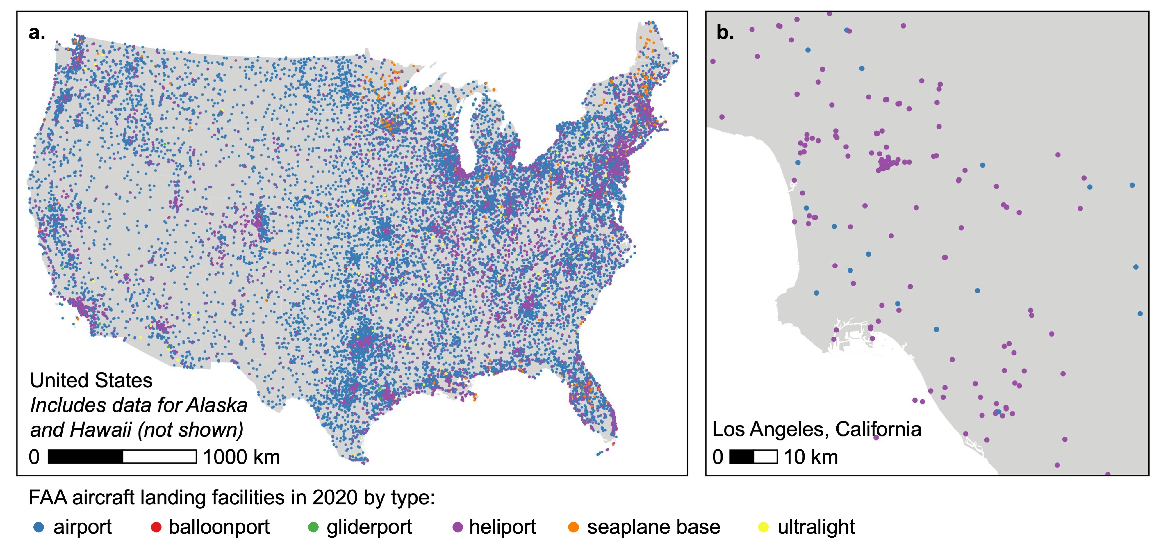
The FAA aircraft landing facility data includes a registry of point locations (i.e., coordinates) of arrival and departure of aircraft in the US. FAA provides the following categorization of aircraft landing facility types: airports, heliports, seaplane bases, gliderports, ultralights, and balloonports. FAA also provides the activation year for facilities starting in year 1981.
The following figure illustrates the spatial coverage (all US states) and spatial scale (points) of the FAA aircraft landing facility data:
Exposure Metrics
This tool calculates proximity-based (i.e., distance-based) exposure metrics for a specified list of receptor point locations (e.g., geocoded home addresses) to aircraft landing facilities in a specified year (during 1981-2020). This tool can be used to calculate the following proximity-based metrics within the US:
- Distance to nearest aircraft landing facility and identity of nearest aircraft landing facility (i.e., identifying codes, facility type, and activation year)
- Count of aircraft landing facilities within a specified buffer distance of receptor
- Summary metrics of distances to all aircraft landing facilities within a specified buffer distance of receptor (i.e., mean distance, mean of logarithm distance, and 25th, 50th, and 75th percentile distances)
Proximity metrics can be calculated for all FAA aircraft landing facility types (i.e., airports, heliports, seaplane bases, gliderports, ultralights, and balloonports) or any subset of them. Output includes information about data missingness (e.g., whether a receptor location is near a US border) as well as an optional log file.
Recommended Uses
This tool is recommended for the following uses:
- Applications for which a proximity-based metric is appropriate. Note: This tool does not provide other relevant exposure information associated with aircraft landing facilities, such as traffic (e.g., annual count of arrivals/departures), noise levels, or air pollution levels.
- Applications for which most receptor point locations are not located near to a US border with Mexico or Canada. Note: Because this tool does not include aircraft landing facility data for Mexico or Canada, the tool may under predict proximity to aircraft landing facilities for receptor point locations in the US near a border with Mexico or Canada with nearby aircraft landing facilities across the border. This tool provides optional output information indicating whether a receptor point is located within a specified distance of a border.
7.3.2 Install R and Required Packages
Install R. Optionally, install RStudio.
Then, install the following R packages: logr, tidyverse, sf.
Follow R package installation instructions, or run the following code in R:
7.3.3 Download Tool
Download and save the folder containing input data (input_source_aircraft_facilities.rds and input_us_borders.rds) and script (script_aircraft_facility_proximity_for_points.R). To directly run the example scripts provided with these instructions in Step 4, do not change the file names within the folder.
7.3.4 Prepare Receptor Point Data
Prepare a comma-separated values (CSV) file that contains a table of the receptor point locations (e.g., geocoded addresses, coordinates). Include each receptor as a separate row in the table, and include the following required columns:
id: a unique and anonymous identifying code for each receptor. This can be in character (string) or numeric (double) format
latitude: the latitude of the receptor point location in decimal degrees format (range: -90 to 90)longitude: the longitude of the receptor point location in decimal degrees format (range: -180 to 180)
The following table provides an example of the receptor point data format:
| id | latitude | longitude |
|---|---|---|
| 1011A | 39.00205369 | -77.105578716 |
| 1012C | 35.88480215 | -78.877942573 |
| 1013E | 39.43560788 | -77.434847823 |
To directly run the example scripts provided with these instructions, save the receptor point data as input_receptor.csv in the folder.
7.3.5 Run Script in R
Run the script script_aircraft_facility_proximity_for_points.R to load the required functions in R. You can then use the function get_aircraft_facility_proximity_for_points() to calculate proximity-based exposure metrics for each receptor point location.
Description of Function get_aircraft_facility_proximity_for_points()
This function takes the receptor point data above and returns a data frame with the receptor identifying code linked to the selected aircraft landing facility proximity metrics for selected aircraft landing facility types and year (during 1981 to 2020) as well as information about data missingness. Optionally, the function also writes a log file in the current R working directory. The function has the following arguments:
Required Arguments
receptor_filepath: specifies the file path to a CSV file containing the receptor point locations (described in Step 3). Note: The format for file paths in R can vary by operating system.
source_aircraft_facilities_filepath: specifies the file path to a RDS file containing a simple features object with the point locations of FAA aircraft landing facilities. This is the fileinput_source_aircraft_facilities.rds.
us_borders_filepath: specifies the file path to a RDS file containing a simple features object with the US borders with Mexico and Canada. This is the fileinput_us_borders.rds.aircraft_year: specifies a single year (in YYYY format; e.g., 2003) for proximity-based exposure assessment across all pollutants. Default isNULL. Year must be during 1981 to 2020. Aircraft landing facilities activated afteraircraft_yearwill be excluded from calculation of the proximity metrics.
Optional Arguments
buffer_distance_km: a numeric argument that specifies the buffer distance (units: kilometers [km]) to use in calculation of buffer-based proximity metrics. Default is10km. Must be between 0.001 km and 1000 km. Note: Larger buffer distance values may result in longer run-times for buffer-based proximity metrics.receptor_crs: a coordinate reference system object (i.e., class iscrsobject in R) for the receptor point locations. Default is"EPSG:4269"(i.e., NAD83).projection_crs: a projected coordinate reference system object (i.e., class iscrsobject in R) for use in exposure assessment. Default is"ESRI:102008"(i.e., North America Albers Equal Area Conic projection).aircraft_facility_type: list that specifies the subset of FAA aircraft landing facility types to include in the exposure assessment. Default is all types:"airport", "heliport", "seaplane base", "gliderport", "ultralight", "balloonport".
proximity_metrics: list that specifies the subset of proximity-based exposure metrics to calculate. Default is all metrics:"distance_to_nearest, "count_in_buffer", "distance_in_buffer"."distance_to_nearest": returns output with distance to nearest aircraft landing facility (units: km) and identity of nearest aircraft landing facility (i.e., identifying codes, facility type, and activation year) for each receptor
"count_in_buffer": returns output with count of aircraft landing facilities within a specified buffer distance of each receptor
"distance_in_buffer": returns output with summary metrics of distances to all aircraft landing facilities within the specified buffer distance of receptor (i.e., mean distance, mean of logarithm distance, and 25th, 50th, and 75th percentile distances to all aircraft landing facilities for each receptor)
check_near_us_border: logical argument that specifies whether the function should identify receptor points that are within the buffer distance (i.e., specified by argumentbuffer_distance_km) of a US border with Canada or Mexico.TRUEreturns a column with output (within_border_buffer) with a binary variable indicating receptor points within the buffer distance of a border. Default isTRUE. Note: The aircraft landing facility data covers only facilities located within the US. Thus, this tool may under predict proximity to aircraft landing facilities for receptor locations near a US border with Canada or Mexico.
add_all_input_to_output: logical argument that specifies whether the output of the function should include all columns included with the input receptor data frame or not.TRUEreturns all columns (i.e., including latitude and longitude) with output.FALSEreturns only the anonymous receptor identifying code, proximity-based metrics, and data missingness information with output.FALSEmay be useful for meeting data de-identification requirements. Default isTRUE.
write_log_to_file: logical argument that specifies whether a log should be written to file.TRUEwill create a log file in the current working directory. Default isTRUE.
print_log_to_console: logical argument that specifies whether a log should be printed to the console.TRUEwill print a log to console. Default isTRUE.
Example Use
Below are two example scripts for using the function above to produce a CSV file with the proximiity-based exposure estimates for each receptor to airports in year 2020 (using default options for all other optional arguments). The first example uses only R but requires editing the file paths. The second example requires RStudio and the here package but does not require editing file paths.
Example 1: Base R
# Load packages
library(tidyverse)
library(logr)
library(sf)

# Load functions
source("/set/file/path/to/script_aircraft_facility_proximity_for_points.R")

# Get exposures
aircraft_proximity_metrics <-
  get_aircraft_facility_proximity_for_points(
    receptor_filepath = "/set/file/path/to/input_receptor.csv",
    source_aircraft_facilities_filepath =
    "/set/file/path/to/input_source_aircraft_facilities.rds",
    us_borders_filepath =
    "/set/file/path/to/input_us_borders.rds",
    aircraft_year = 2020,
    aircraft_facility_type = "airport"
  )

# Write exposures to CSV
readr::write_csv(aircraft_proximity_metrics,
  file = "/set/file/path/to/output_aircraft_proximity_metrics.csv"
)
Example 2: RStudio with here Package
# Install here package (if needed)
install.packages("here")

# Load packages
library(here)
library(tidyverse)
library(logr)
library(sf)

# Set location
here::i_am("script_aircraft_facility_proximity_for_points.R")

# Load functions
source(here::here("script_aircraft_facility_proximity_for_points.R"))

# Get exposures
aircraft_proximity_metrics <-
  get_aircraft_facility_proximity_for_points(
    receptor_filepath = here("input_receptor.csv"),
    source_aircraft_facilities_filepath =
    here("input_source_aircraft_facilities.rds"),
    us_borders_filepath = here("input_us_borders.rds"),
    aircraft_year = 2020,
    aircraft_facility_type = "airport"
  )

# Write exposures to CSV
readr::write_csv(aircraft_proximity_metrics,
  file = here("output_aircraft_proximity_metrics.csv")
)
7.3.6 Review Output
Log File
After running the example script above, with the log file option selected, the log
file will be available in the folder log in the current R working directory.
Output Data
After running the example script above, calculated proximity-based exposure metrics for receptor locations will be available in the file output_aircraft_proximity_metrics.csv within the folder. This CSV file includes a row for each receptor with the following columns (as applicable):
Identifiers
id: the unique and anonymous identifying code for each receptor
Calculated Proximity-Based Exposure Metrics
Nearest Distance Metrics
aircraft_nearest_distance_km: distance (units: km) to the nearest aircraft landing facility
aircraft_nearest_id_site_num: the unique identifying FAA site number for the nearest aircraft landing facility. Consists of a numeric code followed by a letter indicating the aircraft landing facility type. For example, the site number for the Los Angeles International Airport is01818.*A. The FAA site number can be used to link additional types of FAA data (e.g., annual operations) for further analyses.
aircraft_nearest_id_loc: the unique identifying location code for the nearest aircraft landing facility. Consists of a 3 or 4 character alphanumeric code. For example, the location code for the Los Angeles International Airport isLAX. The location code can be used to link additional types of FAA data (e.g., annual operations) for further analyses.
aircraft_nearest_fac_type: the type (i.e., airport, heliport, seaplane base, gliderport, ultralight, and balloonport) of the nearest aircraft landing facilityaircraft_nearest_year_activation: the year of activation of the nearest aircraft landing facility. Activation year is available for all facilities starting in 1981.
Count in Buffer Metrics
aircraft_count_in_buffer: number of aircraft landing facilities within the specified buffer distance of each receptor
Distance in Buffer Metrics
aircraft_mean_distance_in_buffer: mean of distances (units: km) to all aircraft landing facilities within the specified buffer distance of receptor.NAindicates that no landing facilities are within the specified buffer distance of the receptor. Note: In cases with exactly one aircraft landing facility within the specified buffer distance, the value will be the distance to that aircraft landing facility.aircraft_log_mean_distance_in_buffer: mean of logarithm of distances (units: km) to all aircraft landing facilities within the specified buffer distance of receptor.NAindicates that no landing facilities are within the specified buffer distance of the receptor. Note: In cases with exactly one aircraft landing facility within the specified buffer distance, the value will be the logarithm of the distance to that aircraft landing facility.aircraft_p25_distance_in_buffer: 25th percentile of distances (units: km) to all aircraft landing facilities within the specified buffer distance of receptor, for cases with at least 10 aircraft landing facilities within the buffer distance.NAindicates that less than 10 aircraft landing facilities are within the buffer distance.aircraft_p50_distance_in_buffer: 50th percentile (i.e., median) of distances (units: km) to all aircraft landing facilities within the specified buffer distance of receptor, for cases with at least 10 aircraft landing facilities within the buffer distance.NAindicates that less than 10 aircraft landing facilities are within the buffer distance.aircraft_p75_distance_in_buffer: 75th percentile of distances (units: km) to all aircraft landing facilities within the specified buffer distance of receptor, for cases with at least 10 aircraft landing facilities within the buffer distance.NAindicates that less than 10 aircraft landing facilities are within the buffer distance.
Information on Data Missingness
within_border_buffer: binary variable indicating whether receptor point is located within the buffer distance (i.e., specified by argumentbuffer_distance_km) of a US border with Canada or Mexico:1indicates that receptor point is located within the buffer distance of a US border with Canada or Mexico. This indicates that the proximity-based metrics calculated by this tool may represent under predictions of the true proximity-based metrics (i.e., the nearest aircraft landing facility may be located in Canada or Mexico, outside the coverage of the US aircraft landing facility dataset).
0indicates that receptor point is not located within the buffer distance of a US border with Canada or Mexico.
7.3.7 Cite Data and Tool
Please cite the following in any publications based on this tool:
Aircraft Landing Facility Data:
US Federal Aviation Administration (FAA). Airport Data and Information Portal (ADIP). [Available: https://adip.faa.gov/agis/public/#/airportSearch/advanced]. Accessed: April 24, 2022.
Homeland Infrastructure Foundation-Level Data (HIFLD) Geoplatform. Aircraft landing facilities geospatial data. [Available: https://hifld-geoplatform.opendata.arcgis.com/datasets/geoplatform::aircraft-landing-facilities/about]. Accessed: June 23, 2022.
US Borders:
Homeland Infrastructure Foundation-Level Data (HIFLD) Geoplatform. Canada and US border geospatial data. [Available: https://hifld-geoplatform.opendata.arcgis.com/datasets/geoplatform::canada-and-us-border/about]. Accessed: June 23, 2022.
Homeland Infrastructure Foundation-Level Data (HIFLD) Geoplatform. Mexico and US border geospatial data. [Available: https://hifld-geoplatform.opendata.arcgis.com/datasets/geoplatform::mexico-and-us-border/about]. Accessed: June 23, 2022.
NIEHS Geospatial Toolbox:
Citation to be determined.
7.4 Major Road Proximity
The following are step-by-step instructions to calculate proximity-based exposure metrics to major roadways in the United States (US) using US NASA (National Aeronautics and Space Administration) Socioeconomic Data and Applications Center (SEDAC) Global Roads Open Access Data Set (Version 1).
7.4.1 Description
NASA SEDAC Roads Data
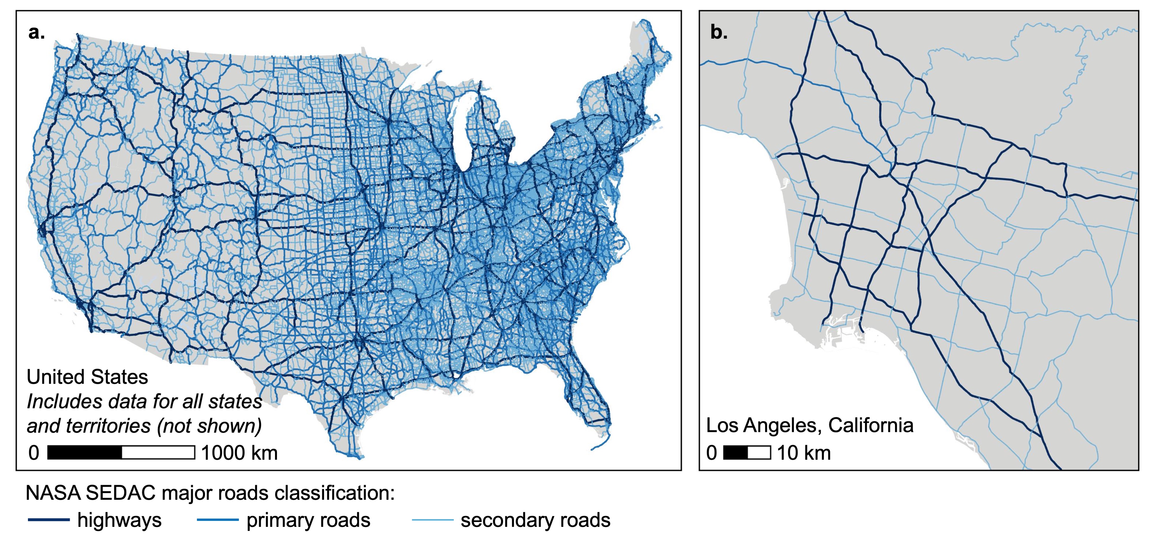
The NASA SEDAC global data includes the locations of major roads (i.e., lines indicating roadway center lines) for the US in 2005. Major roads are categorized based on social and economic importance as follows:
| Major road classification | Description |
|---|---|
| Highways | Limited access divided highways connecting major cities. |
| Primary roads | Other primary major roads between and into major cities as well as primary arterial roads. |
| Secondary roads | Other secondary roads between and into cities as well as secondary arterial roads. |
Other types of roads, such as tertiary roads, local roads, trails, and private roads, are not included.
The following figure illustrates the spatial coverage (all US states and territories) and spatial scale (lines) of the SEDAC roads data:
Exposure Metrics
This tool calculates proximity-based (i.e., distance-based) exposure metrics for a specified list of receptor point locations (e.g., geocoded home addresses) to major roads in year 2005. This tool can be used to calculate the following proximity-based metrics within the US:
- Distance to nearest major road and classification of nearest major road
- Length of road within a specified buffer distance of receptor
These proximity-based metrics can be calculated for all available major road classifications (i.e., highways, primary roads, and secondary roads) or any subset of them. Output includes information about data missingness (e.g., whether a receptor location is near a US border) as well as an optional log file.
Recommended Uses
This tool is recommended for the following uses:
- Applications for which a proximity-based metric is appropriate. Note: This tool does not provide other relevant exposure information associated with roads, such as traffic, noise levels, or air pollution levels.
- Analyses focused on exposures related specifically to major roads. Note: This tool does not include data for other road classifications, such as local street networks or trails.
- Applications for which most receptor point locations are not located in communities with sections of tunneled or elevated highways. Note: This tool does not provide information about whether roads are at surface level (e.g., elevated, tunneled, etc.). Exposure implications of roadway proximity may differ depending on whether road is at surface level. Some urban highways have varying tunneled, surface-level, or elevated sections (e.g., tunneled sections of US Interstate 90 in Boston, Massachusetts, and in Seattle, Washington).
- Applications for which most receptor point locations are not located near to a US border with Mexico or Canada. Note: Because this tool does not include roadway data for Mexico or Canada, the tool may under predict proximity to major roads for receptor point locations in the US near a border with Mexico or Canada with nearby major roads across the border. This tool provides optional output information indicating whether a receptor point is located within a specified distance of a border.
7.4.2 Install R and required packages
Install R. Optionally, install RStudio.
Then, install the following R packages: logr, tidyverse, sf.
Follow R package installation instructions, or run the following code in R:
7.4.3 Download Tool
Download and save the folder containing input data (input_source_major_roads.rds and input_us_borders.rds) and script (script_major_road_proximity_for_points.R). To directly run the example scripts provided with these instructions in Step 4, do not change the file names within the folder.
7.4.4 Prepare Receptor Point Data
Prepare a comma-separated values (CSV) file that contains a table of the receptor point locations (e.g., geocoded addresses, coordinates). Include each receptor as a separate row in the table, and include the following required columns:
id: a unique and anonymous identifying code for each receptor. This can be in character (string) or numeric (double) format
latitude: the latitude of the receptor point location in decimal degrees format (range: -90 to 90)longitude: the longitude of the receptor point location in decimal degrees format (range: -180 to 180)
The following table provides an example of the receptor point data format:
| id | latitude | longitude |
|---|---|---|
| 1011A | 39.00205369 | -77.105578716 |
| 1012C | 35.88480215 | -78.877942573 |
| 1013E | 39.43560788 | -77.434847823 |
To directly run the example scripts provided with these instructions, save the receptor point data as input_receptor.csv in the folder.
7.4.5 Run script in R
Run the script script_major_road_proximity_for_points.R to load the required functions in R. You can then use the function get_major_road_proximity_for_points() to calculate proximity-based exposure metrics for each receptor point location.
Description of Function get_major_road_proximity_for_points()
This function takes the receptor point data above and returns a data frame with the receptor identifying code linked to the selected major road facility proximity metrics for selected raod class(es) as well as information about data missingness. Optionally, the function also writes a log file in the current R working directory. The function has the following arguments:
Required Arguments
receptor_filepath: specifies the file path to a CSV file containing the receptor point locations (described in Step 3). Note: The format for file paths in R can vary by operating system.
source_major_roads_filepath: specifies the file path to a RDS file containing a simple features object with the line locations of NASA SEDAC major roads in the US. This is the fileinput_source_major_roads.rds.
us_borders_filepath: specifies the file path to a RDS file containing a simple features object with the US borders with Mexico and Canada. This is the fileinput_us_borders.rds.
Optional Arguments
buffer_distance_km: a numeric argument that specifies the buffer distance (units: kilometers [km]) to use in calculation of buffer-based proximity metrics. Default is1km. Must be between 0.001 km and 1000 km. Note: Larger buffer distance values may result in longer run-times for buffer-based proximity metrics.receptor_crs: a coordinate reference system object (i.e., class iscrsobject in R) for the receptor point locations. Default is"EPSG:4269"(i.e., NAD83).
projection_crs: a projected coordinate reference system object (i.e., class iscrsobject in R) for use in exposure assessment. Default is"ESRI:102008"(i.e., North America Albers Equal Area Conic projection).road_class_selection: list that specifies the subset of major road types to include in the exposure assessment. Default is all types:"highway", "primary road", "secondary road", "unspecified".
proximity_metrics: list that specifies the subset of proximity-based exposure metrics to calculate. Default is all metrics:"distance_to_nearest, "length_in_buffer"."distance_to_nearest": returns output with distance to nearest major road (units: km) and classification of nearest major road (e.g., highway) for each receptor
"length_in_buffer": returns output with the length (units: km) of all major roads of the selected class(es) within the specified buffer distance of receptor
check_near_us_border: logical argument that specifies whether the function should identify receptor points that are within the buffer distance (i.e., specified by argumentbuffer_distance_km) of a US border with Canada or Mexico.TRUEreturns a column with output (within_border_buffer) with a binary variable indicating receptor points within the buffer distance of a border. Default isTRUE. Note: This tool includes only road data for US states and territories. Thus, this tool may under predict proximity to major roads for receptor locations near a US border with Canada or Mexico.
add_all_input_to_output: logical argument that specifies whether the output of the function should include all columns included with the input receptor data frame or not.TRUEreturns all columns (i.e., including latitude and longitude) with output.FALSEreturns only the anonymous receptor identifying code, proximity-based metrics, and data missingness information with output.FALSEmay be useful for meeting data de-identification requirements. Default isTRUE.
write_log_to_file: logical argument that specifies whether a log should be written to file.TRUEwill create a log file in the current working directory. Default isTRUE.
print_log_to_console: logical argument that specifies whether a log should be printed to the console.TRUEwill print a log to console. Default isTRUE.
Example Use
Below are two example scripts for using the function above to produce a CSV file with the proximity-based exposure estimates for each receptor to highways (using default options for all other optional arguments). The first example uses only R but requires editing the file paths. The second example requires RStudio and the here package but does not require editing file paths.
Example 1: Base R
# Load packages
library(tidyverse)
library(logr)
library(sf)

# Load functions
source("/set/file/path/to/script_major_road_proximity_for_points.R")

# Get proximity-based exposures
major_road_proximity_metrics <-
  get_major_road_proximity_for_points(
    receptor_filepath = "/set/file/path/to/input_receptor.csv",
    source_major_roads_filepath =
    "/set/file/path/to/input_source_major_roads.rds",
    us_borders_filepath =
    "/set/file/path/to/input_us_borders.rds",
    road_class_selection = "highway"
  )

# Write exposures to CSV
readr::write_csv(major_road_proximity_metrics,
  file = "/set/file/path/to/output_major_road_proximity_metrics.csv"
)
Example 2: RStudio with here Package
# Install here package (if needed)
install.packages("here")

# Load packages
library(here)
library(tidyverse)
library(logr)
library(sf)

# Set location
here::i_am("script_major_road_proximity_for_points.R")

# Load functions
source(here::here("script_major_road_proximity_for_points.R"))

# Get exposures
major_road_proximity_metrics <-
  get_major_road_proximity_for_points(
    receptor_filepath = here("input_receptor.csv"),
    source_major_roads_filepath = here("input_source_major_roads.rds"),
    us_borders_filepath = here("input_us_borders.rds"),
    road_class_selection = "highway"
  )

# Write exposures to CSV
readr::write_csv(major_road_proximity_metrics,
  file = here("output_major_road_proximity_metrics.csv")
)
7.4.6 Review Output
Log File
After running the example script above, with the log file option selected, the log
file will be available in the folder log in the current R working directory.
Output Data
After running the example script above, calculated proximity-based exposure metrics for receptor locations will be available in the file output_major_road_proximity_metrics.csv within the folder. This CSV file includes a row for each receptor with the following columns (as applicable):
Identifiers
id: the unique and anonymous identifying code for each receptor
Calculated Proximity-Based Exposure Metrics
Nearest Distance Metrics
major_road_nearest_distance_km: distance (units: km) to the nearest major road
major_road_nearest_road_class: the classification of the nearest major road segment.
Length in Buffer Metrics
major_road_length_in_buffer_km: length (units: km) of all major roads of the specified class(es) within the specified buffer distance of receptor.0indicates that no major roads are within the specified buffer distance of the receptor.
Information on Data Missingness
within_border_buffer: binary variable indicating whether receptor point is located within the buffer distance (i.e., specified by argumentbuffer_distance_km) of a US border with Canada or Mexico:1indicates that receptor point is located within the buffer distance of a US border with Canada or Mexico. This indicates that the proximity-based metrics calculated by this tool may represent under predictions of the true proximity-based metrics (i.e., the nearest major road may be located in Canada or Mexico, outside the coverage of the major road data included in this tool).
0indicates that receptor point is not located within the buffer distance of a US border with Canada or Mexico.
7.4.7 Cite Data and Tool
Please cite the following in any publications based on this tool:
Major Roads Data:
Center for International Earth Science Information Network - CIESIN - Columbia University, and Information Technology Outreach Services - ITOS - University of Georgia. (2013). Global Roads Open Access Data Set, Version 1 (gROADSv1). Palisades, New York: NASA Socioeconomic Data and Applications Center (SEDAC). [Available: https://doi.org/10.7927/H4VD6WCT.] Accessed October 24, 2022.
US Borders:
Homeland Infrastructure Foundation-Level Data (HIFLD) Geoplatform. Canada and US border geospatial data. [Available: https://hifld-geoplatform.opendata.arcgis.com/datasets/geoplatform::canada-and-us-border/about]. Accessed: June 23, 2022.
Homeland Infrastructure Foundation-Level Data (HIFLD) Geoplatform. Mexico and US border geospatial data. [Available: https://hifld-geoplatform.opendata.arcgis.com/datasets/geoplatform::mexico-and-us-border/about]. Accessed: June 23, 2022.
NIEHS Geospatial Toolbox:
Citation to be determined.